
Yelp Dataset Challenge: Sentiment and Business Attributes Analyses
Overview
Two teammates and I worked together on this project.
Our goal is to train the data provided by the Yelp website - specifically the business data on all
existing restaurants in the United States and the reviews written by customers - in order to predict
the relationships between business attributes and the business’ overall success, defined by their star
rating (0-5). In addition to business feature insights, we perform a sentiment analysis using NLP on
the text data provided by customer reviews to help businesses better understand what contributes to
customer preferences. Ultimately, we hope to provide a tool for restaurant owners to predict their
business’ long-run average star rating and to help in their decision-making processes.
Yelp Sentiment and Business Attribute Analysis project was done as the final project of Applied
Machine Learning at Cornell Tech.
Duration
Three months
Programming Language
Python
Role
Data Processing, Feature Extraction Models and Machine Learning Prediction Models for Business Factor Attributes Analysis
Background
Yelp serves as the most popular method to share reviews, photos, and ratings of local restaurants and businesses. These ratings are invaluable information about the quality and performance of a business. They also indicate future popularity as people rely on the star ratings and reviews to make informed decisions about the places to go. Small businesses specifically stand to benefit from this type of rating platform because it helps gain word of mouth traction from a new customer base and also gives them free and invaluable feedback about the performance of their restaurant across a multitude of attributes and categories.
Goals
- Sentiment analysis through using NLP on customer reviews
- Business success prediction model through Feature Extraction Model and Machine Learning Prediction Model
Sentiment Analysis Model
The Dataset
We work with the review json from the Yelp Dataset. This dataset contains the following fields:
Business ID, Review ID, Text, User ID, Userful, Cool, Funny, Date, Stars and Type.
We are specifically working with the ‘text’ and ‘stars’ fields, where ‘stars’ serves as our target
output. We split the training dataset into 70% training, 15% hold-out as a way to obtain accuracy
prior to generalizing our
models. Finally, we test on the remaining 15% of data.
Preprocessing
In order to preprocess the text reviews, we decided to perform the following: (1) remove white spaces,
(2) remove punctuation, (3) remove stop words, and (4) lemmatize words. We also created a new column
called ‘sentiment’
which converts to star ratings into either a positive, neutral or negative review. Ratings of 1 and 2
map to negative, 3 maps to neutral, and 4 and 5 maps to positive.
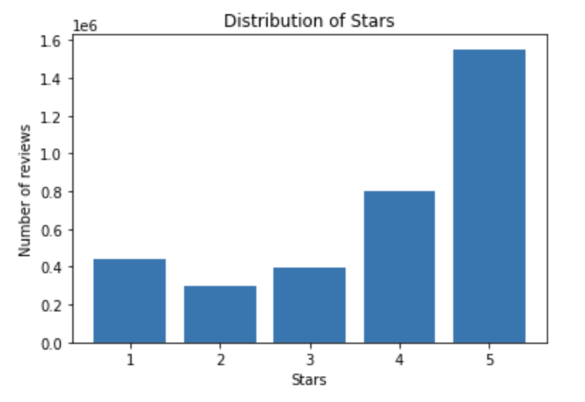
The review data contains 8,021,122 rows of data with the following distribution. We first filtered out
(1) closed businesses, (2) kept only restaurant businesses, and (3) filtered on the businessID’s
contained in the business
dataset. From there our dataset was reduced to 3,487,813 rows and the rating distribution looked like
the following:
Feature Extraction Models
For feature extraction of the text, we use two methods. The first model, the Bag of Words Model, is a representation of text that describes the occurrence of words within a document. It is called a “bag” of words, because any information about the order or structure of words in the document is discarded. The second model, the TF-IDF model, uses a weighting scheme that assigns each term in a document a weight based on its term frequency (tf) and inverse document frequency (idf). The terms with higher weight scores are considered to be more important.
Machine Learning Prediction Models
For the sentiment analysis prediction models, we decided to train on three different models, namely (1) multinomial naive bayes, (2) logistic regression with class set to ‘multinomial’ to account for the different classes in the case of both individual star predictions and sentiment predictions, and (3) linear SVM. For the linear SVM model, we trained the feature vectors on a variety of regularization hyperparameters to find the best classification F1-scores. We graph the F1-scores for each hyperparameter in the following section. These algorithms ultimately allowed us to apply a diverse set of prediction methods for our classification problem and are tailored for text classification.
Experimental Analysis
We ran the multinomial naive bayes, logistic regression, and linear SVM on BoW and TF-IDF on the
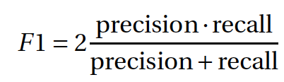
training set and predicted on the hold-out set. After running the models, we use the following
calculation, known as the F1-score, a geometric mean of precision
and recall which represents our ability to predict correct positives, to evaluate our models:
| Model | Precision | Recall | F1 Score |
|---|---|---|---|
| Multinomial NB | 0.575 | 0.591 | 0.580 |
| Logistic | 0.563 | 0.574 | 0.567 |
| Linear SVM | 0.525 | 0.534 | 0.528 |
| Model | Precision | Recall | F1 Score |
|---|---|---|---|
| Multinomial NB | 0.464 | 0.516 | 0.309 |
| Logistic | 0.569 | 0.603 | 0.572 |
| Linear SVM | 0.573 | 0.605 | 0.564 |
| Model | Precision | Recall | F1 Score |
|---|---|---|---|
| Multinomial NB | 0.565 | 0.585 | 0.572 |
| Logistic | 0.554 | 0.568 | 0.559 |
| Linear SVM | 0.546 | 0.567 | 0.552 |
| Model | Precision | Recall | F1 Score |
|---|---|---|---|
| Multinomial NB | 0.497 | 0.535 | 0.339 |
| Logistic | 0.577 | 0.603 | 0.574 |
| Linear SVM | 0.541 | 0.564 | 0.549 |
| Model | Precision | Recall | F1 Score |
|---|---|---|---|
| Multinomial NB | 0.806 | 0.810 | 0.807 |
| Logistic | 0.795 | 0.805 | 0.799 |
| Linear SVM | 0.790 | 0.807 | 0.796 |
| Model | Precision | Recall | F1 Score |
|---|---|---|---|
| Multinomial NB | 0.709 | 0.789 | 0.735 |
| Logistic | 0.795 | 0.805 | 0.799 |
| Linear SVM | 0.790 | 0.807 | 0.796 |
Final Accuracy Score of Bag of Words Model
| Model | Precision | Recall | F1 Score |
|---|---|---|---|
| Multinomial NB | 0.796 | 0.807 | 0.801 |
| Logistic | 0.805 | 0.821 | 0.810 |
| Linear SVM | 0.801 | 0.821 | 0.807 |
Business Attributes Analysis Model
The Dataset
We work with the business json from the Yelp Dataset. Out of all the columns, the ‘city’, ‘state’, ‘postal code’, ‘stars’, ‘review_count’, and ‘attributes‘ fields are used. All other features serve as x, while ‘stars’ serve as y - the target. We split the training dataset into 70% training, 15% hold-out, and the remaining 15% test data.
Preprocessing
In order to preprocess the business data, we took care of the following: (1) missing data, (2) businesses other than restaurants, (3) closed restaurants, and (4) restaurants outside the United States. We also created a new column called ‘binary_star’ that converts ratings into either positive (1) or negative (0). Ratings of 1 and 2 map to negative and 4 and 5 maps to positive.
Feature Extraction Models
All potential business features that could impact the average star rating of the respective restaurant have been extracted. Afterwards, categorical features were converted to binary conditional data of (yes, no).
Machine Learning Prediction Models
For the business factor analysis prediction models, we decided to train on three different models, namely (1) random forest regression, (2) decision tree regression and (3) linear regression. For regression models, we set the target output to be continuous variables. To measure accuracy, the MSE, MAE, RMSE have been used.
Experimental Analysis
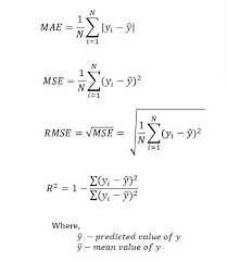
We ran various regression models on the training set and predicted on the hold-out set. After running
the models, we used the mean absolute error (MAE), mean squared error (MSE), and root mean squared error
(RMSE) to evaluate the accuracy of our models:
| Model | Precision | Recall | F1 Score |
|---|---|---|---|
| Linear Regression | 0.537 | 0.464 | 0.681 |
| Logistic Regression | 0.292 | 0.293 | 0.541 |
| Decision Tree Regression | 0.584 | 0.578 | 0.760 |
| Adaboost Regression | 0.551 | 0.475 | 0.690 |
| Random Forest Regression | 0.557 | 0.511 | 0.715 |
Random Forest Regression
For a random forest regressor, we fit to find the best parameters, with which we get the baseline performance: the average error is 0.5526 degree and the accuracy is 81.93%. After fitting on the dev data, its average error has decreased to 0.5216 degrees and its accuracy improved to 82.66%. This is an improvement of 0.90%, which can be significant in respective to a 5-star-rating system.
Decision Tree Regression
For a decision tree regressor, we fit to find the best parameters, with which we got the baseline performance: the average error is 0.5834 degree and the accuracy is 81.16%. After fitting on the dev data, its average error has decreased to 0.5216 degrees and its accuracy improved to 82.66%. This is an improvement of 1.86%, which can be significant in respective to a 5-star-rating system.
Adaboost Regression
The initial prediction of adaboosting on train data is the following: [MAE: 0.5524, MSE: 0.4779, RMSE: 0.6913]. This has been improved to [MAE: 0.5465, MSE: 0.4629, RMSE: 0.6804]
Linear Regression
The initial prediction of adaboosting on train data is the following: [MAE: 0.5320, MSE: 0.4635, RMSE: 0.6808]. While there is no difference in MAE, otherwise this has been improved for MSE to 0.4397 and RMSE to 0.6631.
Discussion
Sentiment Analysis Model
From the experimental results, we can see that: (1) based on the two different feature extraction models, the Bag of Words model generally performed better than the TF-IDF model. (2) There did not seem to be a significant difference between preprocessing the text and no preprocessing of the text and in some cases, preprocessing led to worse performance. After doing more research, this seems plausible since some stop words convey sentiment and thus removing them will decrease the accuracy of the overall models. (4) We also found that within the BoW runs, the logistic regression with multiclass set to multinomial generated the best accuracy performance at an F1 score of 0.810. (5) Some of the top words that contributed to a high rating were ['amaze' 'delicious' 'excellent' 'awesome' 'exactly']. On the other hand, some of the top words that contributed to a poor rating were ['mediocre' 'rude' 'overprice' 'horrible' 'poor']. Thus, we can conclude that there are a number of potential factors at play, such as quality of the food, service, and the overall experience. This information is especially important and salient for restaurant owners because it allows them to gain a better understanding of what factors contribute to a high or low ratings in an easily digestible format. From there, they can adjust their dining options and experience accordingly.
Business Attributes Analysis Model
From the experimental results, we can see that: (1) both Random Forest Regression and Decision Tree models have the potential to much improve with grid search. (2) Random Forest Regression works the best with the number of trees in the forest set to be 600, the minimum number of samples required to split an internal node 10, the minimum number of samples required to be a leaf node 2, the number of features to consider when looking for the best split to be square root, and the maximum depth of the tree 60. (3) The best model performance can be achieved with a criterion of using mean squared error with Friedman’s improvement score for potential splits, the max depth of the tree of 6, and the minimum number of samples required to split an internal node is 2.
Conclusion
In this paper, we explicated multiple machine learning based methods to help business owners expand upon their current suite of resources to better understand their consumer base in terms of both reviews and business attributes. We created two models to achieve this end. The first model, the sentiment analysis model, ran MultinomialNB, logistic regression, and Linear SVM. The second model, the business attributes, ran linear regression, logistic regression, decision tree regression, and random forest regression. Overall, the set of business attributes we tested seem to be reasonable predictors of a restaurant’s average star rating.